
Current transportation planning practices are shifting toward a focus on accessibility – the ease in which a person can reach destinations given the available transportation network – for all modes of transportation including walking, bicycling, and using public transit. This article will explain different methods of measuring accessibility and how to adapt those methods for pedestrian travel. Much previous work on the subject suggests that you need to buy expensive data and software packages like ArcGIS Network Analyst Extension, but free open-source options can provide a suitable alternative. The article will conclude with a walkthrough of using QGIS with data from OpenStreetMaps (OSM) to calculate pedestrian accessibility, using the example of accessibility to restaurants for buildings in the Capitol Complex of St. Paul, Minnesota where I currently work.
Background
What is accessibility?
\”Transportation researchers generally refer to accessibility as a measurement of the spatial distribution of activities about a point, adjusted for the ability and the desire of people or firms to overcome this spatial separation or \’the potential of opportunities of interaction\’ \” (Van Eggermond and Erath 2016). In simpler language, accessibility is a person’s ability to use a transportation network to reach \”opportunities\”, such as jobs, shopping, or recreational activities.
One crucial detail about accessibility is that it is a characteristic of a person or good, and not of a transportation system or mode (Halden et al. 2005). This complicates the measure of accessibility because not everyone has the same preferences and behaviors. For example, consider the major differences between measuring pedestrian accessibility for a senior citizen, a teenager, and a family with children. How far would each of these subjects be willing to walk? What kind of environments would they be willing to walk in? Now realize that this example mostly highlights the difference in age and that there are innumerable cultural, behavioral, and socioeconomic factors that can also change accessibility from person to person.
Accessibility vs. Mobility
The terms accessibility and mobility are often used interchangeably, although they actually represent different concepts. Mobility measures a person’s ability to move between places (Halden et al. 2005; El-Geneidy and Levinson 2006), an indicator of the speed of travel and the robustness of the transportation network. In contrast, accessibility also includes personal preferences and counts the opportunities available.
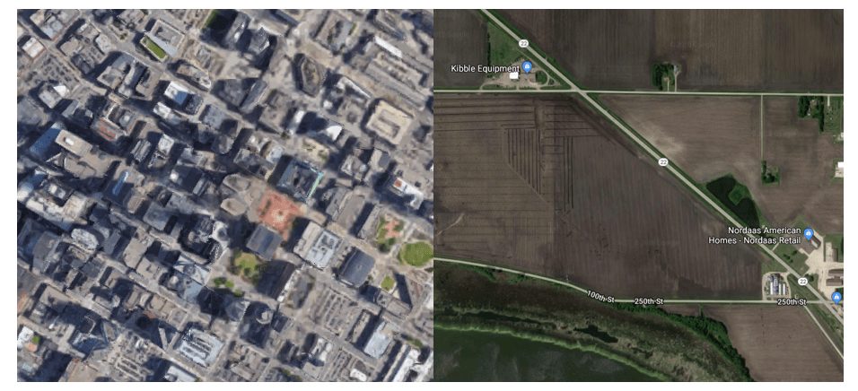
El-Geneidy and Levinson (2006) provide an excellent example illustrating the difference between the two: consider the difference between high density Manhattan and rural Manitoba. In Manhattan, travel speeds are slow due to traffic and many intersections, meaning Manhattan has low mobility. However, the urban density provides numerous opportunities within a short distance, meaning Manhattan has high accessibility. Contrastingly, rural Manitoba has high mobility but low accessibility because most travel occurs on fast highways but there are fewer opportunities with large distances between them.
Halden et al. (2005) discusses how past transportation policy and planning has focused on mobility without much consideration of who is traveling, where they’re going, and what they’re doing at their destination. The authors assert that the problem with emphasizing mobility is that it is unclear whether more or less travel is better and that improved mobility does not necessarily improve accessibility.
Measuring Accessibility
Despite the impossibility of calculating accessibility precisely and accurately for every person, the estimates of a general calculation can provide insights into the built environment and transportation system. In urban planning, accessibility measures can help determine which design for a new subdivision is best, like in the study by Aultman-Hall et al. (1997) which found that building walkways and other pedestrian oriented design choices greatly increase accessibility of a new development. When pairing accessibility measures with demographic data, you can begin to answer questions like \”Do lower income neighborhoods have different levels of accessibility than higher income neighborhoods?\” and the broader question of \”Does the transportation network serve the needs of the population?\”
Accessibility measures have their origins with the development of the Interstate Highway System in the 1950s, when transportation planning first became a serious topic in order to address the growing demand for automobile travel. Traditional practices involved dividing the study area into zones (often referred to as TAZs for transportation analysis zones) and using the transportation network to travel between each zone. Each zone contains a number of opportunities, usually represented by the number of jobs or businesses, which serve as an attraction for travel – a zone with more opportunities is more attractive than a zone with fewer opportunities.
The necessary data for the above mentioned method of accessibility measurement consists of four components: land use, transportation, temporal, and individual (Van Eggermond and Erath 2016). The land use data provides the nodes, the origins and destinations for travel represented as points or zones, and details about the opportunities within a zone, such as number of businesses, etc. The transportation data contains the network: roads and highways for automobiles, bus and train routes for transit, and sidewalks and trails for pedestrians. Temporal data includes roadway speeds (the means to estimate travel time when given a distance), bus and train schedules, and average walking speeds. Individual data approximates personal preferences, such as the maximum distance or time willing to travel for a certain opportunity and the perceived safety of routes.
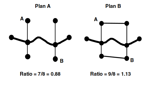
Once data is acquired, measures of mobility are one way of performing an initial assessment of a transportation network. There are four different categories of measurements (May 2014): physical properties such as intersection density, block size, and street layout (grid vs. irregular); street connectivity using the link-to-node ratio (see below illustration); travel-shed to calculate the area within a certain maximum distance; and space syntax, a measure from one point to every other point in an area. Another method similar to the travel-shed would be to create a buffer at a set distance, one as the crow flies (the ideal case) and one using the transportation network (the real case), and then divide the real by the ideal to determine the coverage ratio. Unlike accessibility measures, all of these do not account for personal choice and treat every space in the study area equally — hence the need for accessibility calculations.
The most easily comprehensible method of measuring accessibility simply counts the number of opportunities within an area. The resulting units are tangible, like number of people within walking distance of a business or the number of jobs within walking distance of a neighborhood. This type of analysis is easy in GIS, using one of three methods described by Achuthan et al. (2007): the service area method, similar to walking time maps found in downtowns or tourist areas, which generates polygons for bands of distances calculated using the pedestrian network; the network buffer method, which creates a buffer around the pedestrian network; and the network method, which calculates the distance between one node and all the other nodes using the pedestrian network.
Beyond the above methods, the most commonly used method is the gravity-based measure, which uses a decay function to represent the likelihood of making a trip based on how far the destination is. The basic formula is below, where accessibility equals the sum of the number of opportunities at a destination multiplied by the decay function, usually a negative impedance parameter multiplied by the distance between the origin and opportunity as an exponent of e . The resulting accessibility number has no direct meaning but is useful for comparing areas within the study area.

Other, more complex measures for accessibility exist, but I was unable to find good examples of their use, or like in the case of one method called Miller’s space-time prism, I was unable to comprehend it. Each of the methods above have their advantages and disadvantages, but it is possible to adapt their use for pedestrian travel. However, this is easier said than done and highly dependent on the quality of data available.
Differences Involved When Calculating Pedestrian Accessibility
A major criticism of the existing accessibility literature is that it is automobile-centric (Iacono et al. 2010; Landis et al. 2001; Hoogendoorn and Bovy 2004; Halden et al. 2005; Van Eggermond and Erath 2016; Achuthan et al. 2007; Batty 2001). As such it is necessary to adapt existing studies about automobile accessibility to suitably fit pedestrian scale analysis. In addition, most studies are mainly focused on access to employment (Iacono et al. 2010). This is problematic because most pedestrian trips are for non-work purposes, so any study of pedestrian accessibility should consider opportunities beyond employment.
Adapting Automobile Accessibility Calculations for Pedestrian Use
With automobile trips, travel time is the main determinant (and sometimes the only determinant) of the destination, so assumptions about destination choice can be oversimplified while remaining accurate (Iacono et al. 2010). While directness is often the most important factor when choosing a pedestrian route (pedestrians frequently pick the shortest route but are unaware that is their strategy), other factors complicate the choice such as pleasantness, personal habits, number of crossings, pollution and noise, safety, shelter from weather, and stimulation of environment (Hoogendoorn and Bovy 2004). Cleland and Walton (2004) reviewed several articles studying the reasons people do not walk, finding that the main reasons for not walking were too long of distances, having too much to carry, poor weather conditions, age, health problems and restrictions, and time limitations.
The built environment directly influences travel mode and route choice, with the biggest impact occurring on trips less than one mile (Erath et al. 2016). Looking at past research, Erath et al. saw that sidewalks and other dedicated pedestrian infrastructure had a positive influence on route choice while barriers like crossing a road or parking lot and climbing stairs to an overhead bridge increased the perceived distance. Pedestrians were also likely to take longer routes and detours to use more attractive routes with better scenery and infrastructure. All of these factors make modeling pedestrian behavior especially difficult, partly because some of the considerations in route choice are highly subjective and unmeasurable or lack data at the scale necessary for large scale analysis.
As mentioned previously, the traditional measure of automobile accessibility is the generalization of areas into zones, which is feasible because automobile travel within a zone is minimal (Iacono et al. 2010). However, pedestrian travel encompasses a much smaller geographic footprint and inter-zone travel is common, so analysis requires a coarser resolution than traditional zones provide. Some of the alternatives to zones include building footprints, parcels, and census block groups, the latter of which is particularly useful because of the accompanying demographic data available.
Given the much greater speed and minimal physical effort involved with automobile travel, the impedance function necessary for the accessibility calculation is vastly different for pedestrians. Not only that, but pedestrian behavior is often dependent on the location; pedestrians in New York have much different preferences and tolerances than pedestrians in Los Angeles, not to mention the different behavior between pedestrians in rural, suburban, and urban areas. As such, a localized impedance function is imperative, and luckily (for me) the Minneapolis – St. Paul metro has already been studied. Krizek et al. (2007) developed the following graph showing the distance decay functions for trips for work, shopping, restaurant visits, and entertainment. As illustrated in the graph, people are more willing to walk further for entertainment trips and less willing to walk further for shopping trips. Later I will use the underlying function for the restaurants curve in my walkthrough analysis.

Pedestrian Accessibility Should Focus Less on Employment Trips
The accessibility literature’s focus on employment is problematic because trips for employment account for only a fraction of the total trips a person takes in the day. Take a moment to think about all the trips you take in an average week, where each direction counts as one trip. You’ll probably be surprised at how many trips you take! I quickly estimated mine in the table below, finding that only 34% of my trips are for work, a number that is definitely an overestimate since there are many more non-work trips I take on a less regular basis such as doctor’s appointments, going to the bank, and of course bar crawls that would greatly inflate my social trips.
| Trip Purpose | # of Trips |
| Work | 8 |
| Groceries | 2 |
| Social | 6 |
| Exercise | 6 |
| Shopping | 1 |
| Total | 23 |
| % of work trips | 34% |
Anecdotal evidence aside, real studies have found similar results. The Twin Cities Travel Behavior Inventory conducted in 2010 studied the travel habits of households in the Minneapolis-St. Paul metropolitan area of Minnesota, concluding that only 17% of all trips taken are for work. Furthermore, it found an average household of working adults who are not in school and do not have children takes 6 trips per day, and an average household with children takes 14 trips per day – even if a family had two income earning adults working every day of the week, the four daily work commuting trips still wouldn’t account for a majority of trips.
On a national scale, the National Household Travel Survey in 2009 found that the average person took 3 trips per day – note this includes people of all ages, not just working adults. In addition, an average household took 541 trips to work out of 3,466 total trips in a year or 16% of trips, comparable to the results found in the Twin Cities Travel Behavior Inventory. The American Time Use Survey from 2016 found that the average full time working adult works on average 8.15 hours on 72.5% of days in a week, only slightly higher than the standard 8 hour, 5 day a week schedule. Even out of all employed people holding multiple jobs, 81.8% had at least one day off per week. This presence of \”leisure time\” (in quotes because much of that time might be spent running errands) means plenty of non-work trips.
Not only are the majority of all total trips regardless of mode choice taken for non-work purposes, when looking at pedestrian trips, this majority greatly increases. Again looking at the 2009 National Household Travel Survey, even though pedestrian travel accounts for only 10.4% of all trips, 94% of all pedestrian trips are taken for non-work purposes. This makes sense because the number of job opportunities within reasonable walking distance are minimal unless you live in the dense inner core of a major metropolitan area (or if you talk to your \”15 miles uphill both ways in the snow\” grandfather). As such, analysis of pedestrian accessibility must consider non-work trips a priority.
Walkscore and the Need for Quality Data
Walkscore.com has developed one well-known measure of pedestrian accessibility, mapping areas in major cities where one can accomplish daily tasks easily using walking as the primary means of transportation. The main difficulty in creating such a measurement is the need for highly accurate, detailed data locating the various destinations and the number of jobs, stores, and other information to describe that particular location. This is problematic because data for land use and other variables to help determine route choice are often unavailable at the fine-grained scale necessary or are prohibitively expensive — while Walkscore can afford to pay, nonprofits and government organizations might not have the budget unless doing a massive project. Thus, for small scale analysis at the neighborhood level, it is cost effective to manually create some of the data necessary, but for a larger area such as an entire city this becomes a time consuming and tedious task. Free and open-source data such as that provided by OpenStreetMaps is one potential option to cover a large area with sufficient detail.
Calculating Accessibility with QGIS and OpenStreetMaps (OSM) Data
Now that you understand the basics of accessibility calculations and how to adapt the commonly-used methods for pedestrian analysis, I will detail how you can use the free open-source QGIS to perform accessibility analysis.
Downloading OpenStreetMaps Data
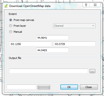
QGIS was designed to work harmoniously with OpenStreetMaps (OSM) and has a built in function to download OSM data. On the menu bar at the top click Vector > OpenStreetMap > Download Data and the window below will pop up. You can specify the extent using the map window, a layer, or manually if you know the bounding coordinates.
Other internet sources provide downloads with preprocessed data and data encompassing entire metropolitan areas or other geographies. If you’re unfamiliar with the structure of OSM data, preprocessed data will be easier to use and will require fewer and less complicated queries to extract what you need.
Creating the Network and Nodes
The step to create the network is the most time consuming part of the process. First you need to extract all of the lines from the OSM data that comprise the pedestrian network, including the lines for roadways and excluding lines for highways and other places that restrict or prohibit pedestrian travel. OSM data also has lines for pedestrian paths and trails, but this data is most likely incomplete and any sidewalk data will duplicate much of the roadway data with the added disadvantage that the sidewalks don’t typically connect at intersections (not ideal when creating a network). As such, it might be easier to manually add pedestrian infrastructure like bridges and park trails than to remove duplicate data and to attempt to verify the accuracy of OSM pedestrian data. In the small study area I used for my example, I decided that the pedestrian infrastructure was not worth including since it added little value compared to the amount of effort it would have required to extract from OSM data or develop my own – I felt the street network was more than adequate for this scenario.
Now you have a network, it’s time to create your dataset of nodes, all the origins and destinations you wish to analyze. This is where you have to be creative, and the nodes you use are dependent on the question you wish to answer. The important thing with this dataset is that you a bunch of points each with its own unique ID that you can later use to join fields with at a later time for deeper analysis.
Traditional transportation analysis uses zones (usually referred to as TAZs), a manufactured boundary that represents a neighborhood unit where the grand assumption is that people within these zones have similar behavior; in this case, you would use the centroid of each zone as a node. Generally these zones are too large to accurately assess pedestrian activity, so parcel centroids are a finer-grained alternative. Centroids of building footprints would be even better, but this data is not widely available, although OSM does have a good number of building footprints especially in major cities. As mentioned previously, census block groups are especially nice to use if you desire to do any sort of demographic analysis in combination with accessibility.
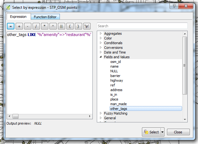
For my particular example, I extracted points tagged with “restaurant” or “fast food” from the OSM points dataset (see query window pictured below) and manually created points for each government building using my own knowledge and aerial imagery. Again, a caveat of using OSM data is that it may be incomplete and you may want to add points for glaring omissions (or even better, log on to OSM and add them there). For example, I noticed an infamous White Castle missing from the OSM restaurant data, so I manually added it. Manual additions may or may not be feasible depending on the size of your study area and the number of nodes under consideration.
Preparing the Data
Since distance calculations are the core of any accessibility analysis, it is essential that your spatial data is in a projected coordinate system. By default, OSM data is in the unprojected WGS84 geographic coordinate system, so you will have to reproject the data to a UTM, state plane, or other projected coordinate system appropriate for the study area.
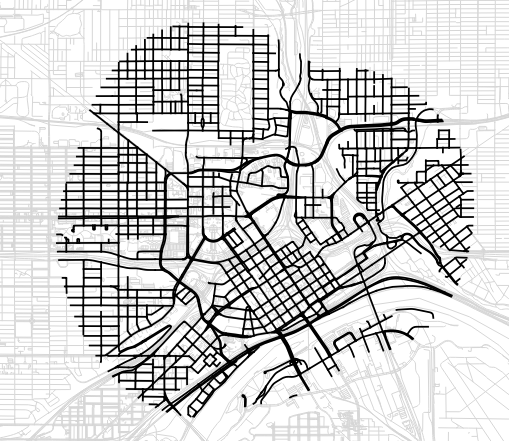
To improve processing performance, I suggest clipping the data to eliminate unnecessary areas outside of the study area. If you’re analyzing overall accessibility within a particular city or metro area, clip using the administrative boundaries. For more localized analysis, such as calculating the pedestrian accessibility to your business, create a buffer around your business location(s) with a distance representing the maximum someone would be willing to walk (around 1.5 miles depending on the study you read and the trip purpose) – since this buffer distance is as the crow flies, it is more than enough to cover the area you need considering that travel is confined to the network. I used this latter method, pictured below, by creating a 1.5 mile buffer around all the buildings in the Capitol Complex.
Once everything is reprojected and clipped properly, you must check the topology of the network and make automatic and manual corrections. This step is especially important when using OSM data because adherence to topology rules is inherently less prevalent given the open nature of the data. If you do not fix topology errors, you will likely receive strange results due to bad connections in the network.
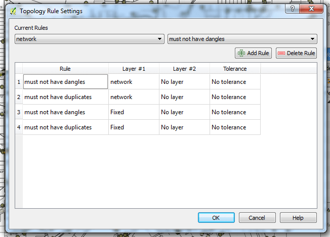
Luckily, the process of fixing topology is relatively straightforward, and I followed the instructions in these PowerPoint slides to learn how to fix topology errors and run network analysis tools in QGIS. First you will have to install the topology checker plugin using the plugin manager in QGIS. Next, open the topology rules window shown below and add the topology rules \”must not have dangles\” and \”must not have duplicates\” on your network layer.
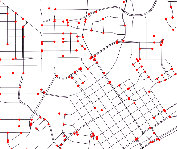
Topology errors will appear on the map as red dots (assuming you have the box checked to show them on the map), and a list of errors will appear alongside. If your data is anything like mine, there will be quite a few! Luckily there is an automatic process you can use to fix most of these errors.
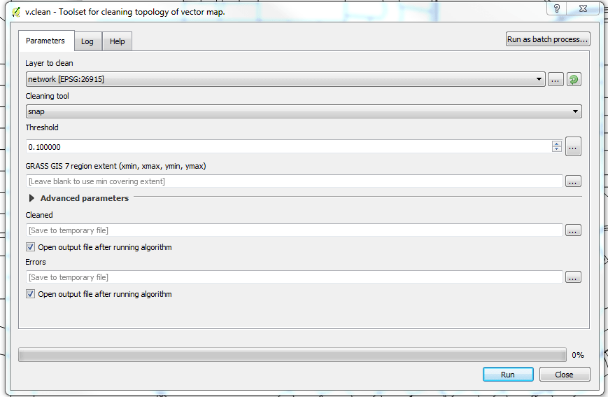
You will then run the v.clean tool in the GRASS toolbox three times using each of these cleaning tools as a parameter: snap, break, and remove dangles; this process ensures all lines in the network are snapped to each other and connected at intersections.
After running the v.clean tool, recheck the topology and you will find the errors have decreased. Now you must manually check all the errors to make sure the v.clean tool didn’t miss anything major – note that some dangles are fine such as with a cul-de-sac or dead end road.
Calculating Accessibility
Once you have both your nodes and your network data, you can begin by calculating the network distance between each pair of nodes using the v.net.allpairs tool in the GRASS toolbox. The inputs are simple: the network layer, the nodes layer, a threshold distance in map units, and an output file destination.
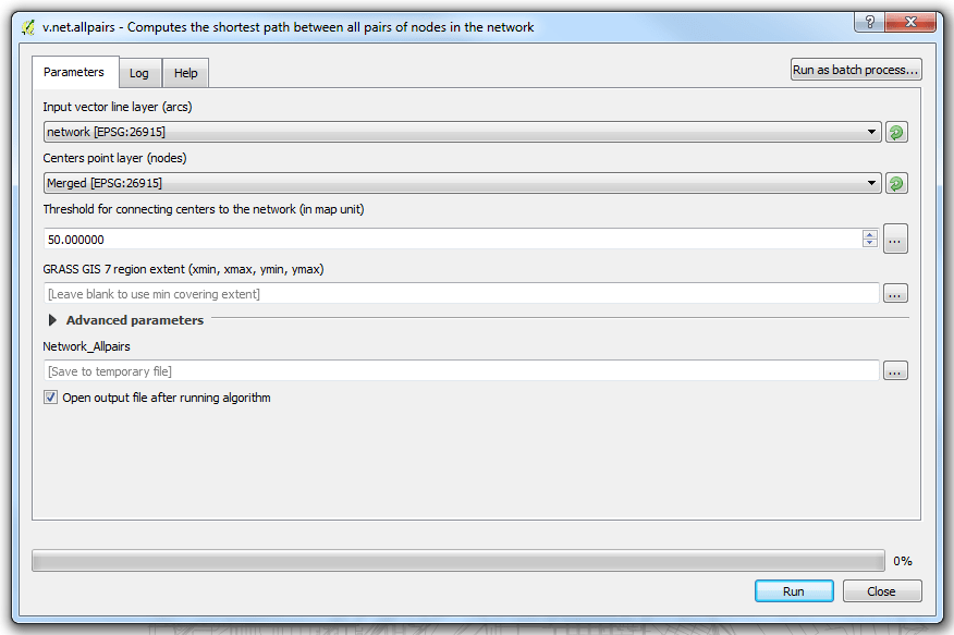
The output of this tool is a line dataset with a simple attribute table consisting of the ID of the origin, ID of the destination, and the distance in map units (again why it’s important that you reproject your data). Surprisingly, it’s easiest to do the rest of the calculations in Excel, so export the attribute table as a CSV – simply right click the layer, click “Save As” and select CSV as the format.
If you remember the formula for accessibility from the background section earlier, the next steps will seem straightforward. If you have trouble understanding math, this process will seem really complicated but if you follow step by step it will give you a beautiful result that you can understand. Now that we have the distances between every pair of nodes, we can calculate the distance decay value, essentially a person’s willingness to walk to a destination given how far away it is. When using a distance decay function from another study, be sure to use the same units! If the output distance calculations use small units like feet or meters due to the projection of your data, you might need to first convert to miles or kilometers or the distance decay function will look like it returns zero for every distance because the resulting calculations will be so small (I ran into this problem the first time).
Since I am interested in trips to restaurants, the Krizek et al. (2007) study provides the specific distance decay function for pedestrians traveling to restaurants, which I\’ve translated into an Excel formula: \”=0.3878*EXP(-1.3919*[distance cell location])\”. Drag this formula to calculate it for every origin/destination pair. Adapt the numbers for your specific scenario and location as necessary.
Now let’s recall the accessibility formula:
Since I used the exact point location of each restaurant rather than a zone, the number of opportunities at the destination is always 1; if your scenario involves multiple opportunities at a single destination, you must first multiply your distance decay function by the number of opportunities. In either case, the easiest way to calculate the sum of the distance decay for each origin point is to use a pivot table. Copy and paste the values from the pivot table, and bam, you have your accessibility measure!
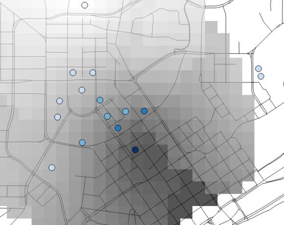
Finally, you can export the accessibility measures as a CSV and join the table back to the nodes dataset using the unique ID field. Now that you have the measures in GIS, you can start making maps and doing other analysis using demographic data, etc. as I have below.

You can also create an accessibility surface using the kriging function in the SAGA toolbox (I\’m not going to explain how to do this because I\’m not sure I entirely understand it well enough myself — looks cool though).
Conclusions
Accessibility is a more comprehensive method to determine the effectiveness of a transportation network, accounting not only for the ability of the system to transport people to places but also for the underlying reasons for travel and the personal preferences and behaviors of the users of the system. While traditionally accessibility studies have focused on automobile travel for work commutes, the methods used are adaptable to other modes of travel. Pedestrian accessibility calculations require fine-grained data and specialized distance decay functions with a greater focus on non-work trip purposes.
The need for high quality data and specialized network analysis tools doesn’t have to mean a large budget, and free open source data via OpenStreetMaps and software via QGIS are available to accomplish the task at hand. Although the underlying math may seem complicated, the actual process is straightforward and provides easily comprehensible results. And finally as for my particular accessibility example, I can conclude that my building has pretty mediocre accessibility to restaurants, mathematically confirming why I haven\’t ventured out for lunch more than a handful of times.
References
Achuthan, Kamalasudhan, Helena Titheridge, and Roger Mackett. 2007. “Measuring Pedestrian Accessibility.” Proceedings of the Geographical Information Science Research UK (GISRUK) Conference. Maynooth, Ireland.
Aultman-Hall, Lisa, Matthew Roorda, and Brian W. Baetz. 1997. “Using GIS for Evaluation of Neighborhood Pedestrian Accessibility.” Journal of Urban Planning and Development 123 (1): 10-17.
Batty, Michael. 2001. “Agent-based Pedestrian Modeling.” Environment and Planning B: Planning and Design 28: 321-326.
Cleland, Bryce S., and Darren Walton. 2004. Why don’t people walk and cycle? New Zealand: Opus International Consultants Limited.
El-Geneidy, Ahmed M., and David M. Levinson. 2006. Access to Destinations: Development of Accessibility Measures. Final Report, St. Paul, Minnesota: Minnesota Department of Transportation.
Erath, Alexander, Michael A.B. van Eggermond, Sergio A. Ordóñez, and Kay W. Axhausen. 2017. “Introducing the Pedestrian Accessibility Tool: Walkability Analysis for a Geographic Information System.” Transportation Research Record: Journal of the Transportation Research Board 2661: 51-61.
Foda, Mohamed A., and Ahmed O. Osman. 2010. “Using GIS for Measuring Transit Stop Accessibility Considering Actual Pedestrian Road Network.” Journal of Public Transportation 13 (4): 23-40.
Halden, Derek, Peter Jones, and Sarah Wixey. 2005. “Accessibility Analysis Literature Review: Measuring accessibility as experienced by different socially disadvantaged groups, Working Paper 3.”
Hale, R.J. n.d. \”Generating Drive Times in GRASS 7.0.4 and QGIS 2.14.3.\” North River Geographic.
Hoogendoorn, S.P., and P.H.L. Bovy. 2004. “Pedestrian route-choice and activity scheduling theory and models.” Transportation Research Part B 38: 169-190.
Iacono, Michael, Kevin J. Krizek, and Ahmed El-Geneidy. 2010. “Measuring non-motorized accessibility: Issues, alternatives, and execution.” Journal of Transport Geography 18: 133-140.
Iacono, Michael, Kevin Krizek, and Ahmed El-Geneidy. 2008. Access to Destinations: How Close is Close Enough? Estimating Accurate Distance Decay Functions for Multiple Modes and Different Purposes. Final Report, St. Paul, Minnesota: Minnesota Department of Transportation.
Krizek, Kevin J., Ahmed El-Geneidy, Michael Iacono, and Jessica Horning. 2007. Access to Destinations: Refining Methods for Calculating Non-Auto Travel Times. Final Report, St. Paul, Minnesota: Minnesota Department of Transportation.
Krizek, Kevin J., Michael Iacono, Ahmed El-Geneidy, Chen Fu Liao, and Robert Johns. 2009. Access to Destinations: Application of Accessbilitiy Measures for Non-Auto Travel Modes. Final Report, St. Paul, Minnesota: Minnesota Department of Transportation.
Landis, Bruce W., Venkat R. Vattikuti, Russell M. Ottenberg, Douglas S. McLeod, and Martin Guttenplan. 2001. “Modeling the Roadside Walking Environment: Pedestrian Level of Service.” Transportation Research Record 1773: 82-88.
May, Douglas. 2016. Pedestrian Disconnect Across Downtown Highways. Graduate Thesis, Manhattan, Kansas: Kansas State University.
Metropolitan Council. 2013. \”Travel Behavior: A Summary of Resident Travel in the Twin Cities Region.\” St. Paul, Minnesota.
U.S. Department of Transportation. 2009. “National Household Travel Survey.” Washington, DC.
van Eggermond, Michael A.B., and Alex Erath. 2016. “Pedestrian and transit accessibility on a micro level: Results and challenges.” The Journal of Transport and Land Use 9 (3): 127-143.
2009 National Household Travel Survey http://nhts.ornl.gov/2009/pub/stt.pdf
2016 American Time Use Survey. https://www.bls.gov/news.release/atus.t03.htm
Comments
One response to “Analyzing Pedestrian Accessibility Using QGIS and OpenStreetMaps Data”
Reblogged this on Dosen GIS and commented:
tag TODO …